Overview
The three main parts of the package are the wtphm.batch, and
wtphm.pred_processing modules, as well as the
wtphm.clustering subpackage.
wtphm.batch contains the functions for creating the batches of
turbine alarms and assigning a high-level reason for the stoppage, gleaned from
the events and scada data. More information on this can be found in [1].
wtphm.pred_processing contains functions for labelling SCADA data based
on the batches, for purposes of fault detection or prognosis.
wtphm.clustering deals with clustering together different similar
alarm sequences, explored in [2]. This part of the library isn’t updated as much
as the others - development may be needed in some parts.
Information and critiques on some of the issues surrounding the data coming from wind turbines more generally can be found in [3].
Input Data Needed for Batch Creation
Batches are groups of turbine events generated by the alarm system which appear during a stoppage. The data to be used for creating the batches and assigning a high level cause for the stop must have certain features, described here.
Events Data
The event_data is related to any fault or information messages generated by
the turbine. This is instantaneous, and records information like faults that have
occurred, or status messages like low- or no- wind, or turbine shutting down due
to storm winds.
The data must have the following column headers and information available:
turbine_num: The turbine the data applies tocode: There are a set list of events which can occur on the turbine. Each one of these has an event codedescription: Each event code also has an associated descriptiontime_on: The start time of the eventstop_cat: This is a category for events which cause the turbine to come to a stop. It could be the functional location of where in the turbine the event originated (e.g. pitch system), a category for grid-related events, that the turbine is down for testing or maintenance, in curtailment due to shadow flicker, etc.- In addition, there must be a specific event
codewhich signifies return to normal operation after any downtime or abnormal operating period.
SCADA Data
The scada_data is typically recorded in 10-minute intervals and has attributes like
average power output, maximum, minimum and average windspeeds, etc. over the previous
10-minute period.
For the purposes of this library, it must have the following column headers and data:
turbine_num: The turbine the data applies totime: The 10-minute period the data belongs to- availability counters: Some of the functions for giving the batches a stop category rely on availability counters. These are sometimes stored as part of scada data, and sometimes in separate availability data. They count the portion of time the turbine was in some mode of operation in each 10-minute period, for availability calculations. For example, maintenance time, fault time, etc. In order to be used in this library, the availability counters are assumed to range between 0 and n in each period, where n is some arbitrary maximum (typically 600, for the 600 seconds in the 10-minute period).
Sample Data
There is sample data provided in the
examples folder of the
github repository. This is 2 months’ of real data for 2 turbines,
but has been fully anonymised. For the event_data, all codes have been
mapped to a random set of numbers, and descriptions have been removed.
For the scada_data, all values have been normalised between 0 and 1,
with the exception of the availability counters (“lot”,
“rt”, etc.) and features counting the number and duration of alarms in the
past 48 hours, “num_48h” and “dur_48h”).
The data can be imported like so:
>>> import wtphm
>>> import pandas as pd
>>> event_data = pd.read_csv('examples/event_data.csv',
...                          parse_dates=['time_on', 'time_off'])
>>> event_data.duration = pd.to_timedelta(event_data.duration)
>>> scada_data  = pd.read_csv('examples/scada_data.csv',
...                           parse_dates=['time'])
>>> event_data.head()
   turbine_num  code             time_on            time_off        duration  stop_cat             description
0           22     9 2015-11-01 00:03:56 2015-11-01 00:23:56 0 days 00:20:00        ok  description anonymised
1           21    93 2015-11-01 00:09:54 2015-11-01 00:10:56 0 days 00:01:02        ok  description anonymised
2           21    97 2015-11-01 00:10:56 2015-11-01 00:37:39 0 days 00:26:43        ok  description anonymised
3           22   165 2015-11-01 00:16:39 2015-11-06 05:03:35 5 days 04:46:56        ok  description anonymised
4           22    93 2015-11-01 00:23:56 2015-11-01 00:24:58 0 days 00:01:02        ok  description anonymised
>>> scada_data.head()
                time  turbine_num  wind_speed        kw  wind_speed_sd  wind_speed_max  ...  lot  wot  est   mt   rt  eect
0 2015-11-01 00:00:00           22    0.148473  0.009655       0.064693        0.110283  ...  0.0  0.0  0.0  0.0  0.0   0.0
1 2015-11-01 00:10:00           22    0.125081  0.004962       0.066886        0.084016  ...  0.0  0.0  0.0  0.0  0.0   0.0
2 2015-11-01 00:20:00           22    0.121183  0.004913       0.060307        0.086624  ...  0.0  0.0  0.0  0.0  0.0   0.0
3 2015-11-01 00:30:00           22    0.137752  0.004454       0.067982        0.104322  ...  0.0  0.0  0.0  0.0  0.0   0.0
4 2015-11-01 00:40:00           22    0.171540  0.040889       0.066886        0.113077  ...  0.0  0.0  0.0  0.0  0.0   0.0
[5 rows x 22 columns]
Group Faults of the Same Type
Sometimes it is useful to treat similar types of fault together as the same type of fault. An example would be faults across different pitch motors on different turbine blades being grouped as the same type of fault. This is useful, as there are typically very few fault samples on wind turbines, so treating these as three separate types of faults would give even fewer samples for each class.
The wtphm.batch.get_grouped_event_data() function does this.
For the pitch fault example above, the grouping would give the events “pitch
thyristor 1 fault” with code 501,
“pitch thyristor 2 fault” with code 502 and “pitch thyristor 3 fault”
with code 503 all the same event description and code, i.e. they all
become “pitch thyristor 1/2/3 fault (original codes 501/502/503)” with
code 501. Note that this is an entirely optional step before creating the
batches of events.
>>> # codes that cause the turbine to come to a stop
... stop_codes = event_data[
...     (event_data.stop_cat.isin(['maintenance', 'test', 'sensor', 'grid'])) |
...     (event_data.stop_cat.str.contains('fault'))].code.unique()
>>> # each of these lists represents a set of pitch-related events, where
... # each memeber of the set represents the same event but along a
... # different blade axis
... pitch_code_groups = [[300, 301, 302], [400, 401], [500, 501, 502],
...                      [600, 601], [700, 701, 702]]
>>> event_data[event_data.code.isin(
...     [i for s in pitch_code_groups for i in s])].head()
     turbine_num  code             time_on            time_off duration  stop_cat                          description
112           22   502 2015-11-01 21:04:26 2015-11-01 21:04:36 00:00:10  fault_pt  description anonymised pitch axis 3
114           22   601 2015-11-01 21:04:28 2015-11-01 21:04:36 00:00:08  fault_pt  description anonymised pitch axis 2
119           22   601 2015-11-01 21:04:36 2015-11-01 21:04:36 00:00:00  fault_pt  description anonymised pitch axis 2
131           22   600 2015-11-01 21:04:36 2015-11-01 21:04:36 00:00:00  fault_pt  description anonymised pitch axis 1
132           22   600 2015-11-01 21:04:36 2015-11-01 21:04:36 00:00:00  fault_pt  description anonymised pitch axis 1
As can be seen, the events data has a number of different codes for data along different pitch axes.
Below, we group these together as the same code (note the descriptions have been anonymised):
>>> event_data, stop_codes = wtphm.batch.get_grouped_event_data(
...     event_data=event_data, code_groups=pitch_code_groups,
...     fault_codes=stop_codes)
>>> # viewing the now-grouped events from above:
... event_data.loc[[112, 114, 119, 131, 132]]
     turbine_num  code             time_on            time_off duration  stop_cat                                                           description
112           22   500 2015-11-01 21:04:26 2015-11-01 21:04:36 00:00:10  fault_pt  description anonymised pitch axis 1/2/3 (original codes 500/501/502)
114           22   600 2015-11-01 21:04:28 2015-11-01 21:04:36 00:00:08  fault_pt        description anonymised pitch axis 1/2 (original codes 600/601)
119           22   600 2015-11-01 21:04:36 2015-11-01 21:04:36 00:00:00  fault_pt        description anonymised pitch axis 1/2 (original codes 600/601)
131           22   600 2015-11-01 21:04:36 2015-11-01 21:04:36 00:00:00  fault_pt        description anonymised pitch axis 1/2 (original codes 600/601)
132           22   600 2015-11-01 21:04:36 2015-11-01 21:04:36 00:00:00  fault_pt        description anonymised pitch axis 1/2 (original codes 600/601)
Creating Batches
As mentioned in [4], turbine alarms often occur in “showers” which can
overwhelm operators and make it difficult to pinpoint the root cause of a
stoppage.
wtphm.batch.get_batch_data() creates the batches. The algorithm is as
follows, as described in detail in [1]:
- A list of event codes which causes the turbine to stop,
fault_codes, are passed to the function, as well as the code which signifies the turbine returning to normal operation after downtime,ok_code. - The earliest event in the
event_datawhich matches a code infault_codesis gotten. Every event between then and the next earliestok_codeevent are stored as a batch. - The next earliest event in
event_datawhich matches a code infault_codesis gotten. Every event between then and the next earliestok_codeevent are stored as a batch, etc.
>>> # create the batches
... batch_data = wtphm.batch.get_batch_data(
...     event_data=event_data, fault_codes=stop_codes, ok_code=207,
...     t_sep_lim='1 hours')
>>> batch_data.loc[15:20]
    turbine_num   fault_root_codes     all_root_codes         start_time  ... fault_dur down_dur    fault_event_ids      all_event_ids
15           22     (68, 113, 500)     (68, 113, 500) 2015-12-03 12:1...  ...  00:03:20 00:07:25  Int64Index([29...  Int64Index([29...
16           22         (144, 500)         (144, 500) 2015-12-08 16:3...  ...  00:11:50 00:15:55  Int64Index([32...  Int64Index([32...
17           22              (73,)          (73, 141) 2015-12-10 18:1...  ...  00:00:00 00:00:17  Int64Index([33...  Int64Index([33...
18           22      (77, 85, 164)      (77, 85, 164) 2015-12-11 10:0...  ...  03:03:14 03:07:25  Int64Index([34...  Int64Index([34...
19           22      (77, 85, 164)      (77, 85, 164) 2015-12-14 12:3...  ...  09:52:49 09:52:51  Int64Index([36...  Int64Index([36...
20           22  (68, 113, 144,...  (68, 113, 144,... 2015-12-16 10:0...  ...  01:09:01 01:09:02  Int64Index([38...  Int64Index([38...
[6 rows x 10 columns]
Note that if two stoppages occur in quick succession, i.e. one batch ends and
another quickly begins, the t_sep_lim argument in
wtphm.batch.get_batch_data() allows us to treat both as the same
continuous batch. For more information about the various columns and parameters,
see the wtphm.batch.get_batch_data() documentation.
Below, we view one of the batches and the event behind it in a bit more detail:
>>> batch_data.loc[20]
turbine_num                               22
fault_root_codes         (68, 113, 144, 500)
all_root_codes           (68, 113, 144, 500)
start_time               2015-12-16 10:00:05
fault_end_time           2015-12-16 11:09:06
down_end_time            2015-12-16 11:09:07
fault_dur                    0 days 01:09:01
down_dur                     0 days 01:09:02
fault_event_ids     Int64Index([3868, 386...
all_event_ids       Int64Index([3868, 386...
Name: 20, dtype: object
>>> event_data.loc[batch_data.loc[20, 'all_event_ids']].head()
      turbine_num  code             time_on            time_off duration  stop_cat                                                           description
3868           22   144 2015-12-16 10:00:05 2015-12-16 10:00:13 00:00:08  fault_pt                                                description anonymised
3867           22    68 2015-12-16 10:00:05 2015-12-16 10:00:13 00:00:08  fault_pt                                                description anonymised
3866           22   500 2015-12-16 10:00:05 2015-12-16 10:00:13 00:00:08  fault_pt  description anonymised pitch axis 1/2/3 (original codes 500/501/502)
3865           22   113 2015-12-16 10:00:05 2015-12-16 10:00:13 00:00:08  fault_pt                                                description anonymised
3869           22   300 2015-12-16 10:00:10 2015-12-16 10:00:13 00:00:03  fault_pt  description anonymised pitch axis 1/2/3 (original codes 300/301/302)
We can also see the corresponding SCADA data. Note that the down-time counter, ‘dt’, which count the number of seconds in each 10-minute period the turbine was down, is active after the start time of the batch, and goes back to zero after it reactivates.
>>> start = batch_data.loc[20, 'start_time'] - pd.Timedelta('20 minutes')
>>> end = batch_data.loc[20, 'down_end_time'] + pd.Timedelta('20 minutes')
>>> t = batch_data.loc[20, 'turbine_num']
>>> scada_data.loc[
...     (scada_data.time >= start) & (scada_data.time <= end) &
...     (scada_data.turbine_num == t),
...     ['time', 'turbine_num', 'wind_speed', 'kw', 'ot', 'sot', 'dt']]
                    time  turbine_num  wind_speed        kw     ot    sot     dt
6425 2015-12-16 09:50:00           22    0.245289  0.298111  600.0  600.0    0.0
6426 2015-12-16 10:00:00           22    0.281027  0.454494  600.0  600.0    0.0
6427 2015-12-16 10:10:00           22    0.263158  0.016645   11.0    6.0  594.0
6428 2015-12-16 10:20:00           22    0.226446  0.005421    0.0    0.0  600.0
6429 2015-12-16 10:30:00           22    0.217674  0.004993    0.0    0.0  600.0
6430 2015-12-16 10:40:00           22    0.195257  0.004906    0.0    0.0  600.0
6431 2015-12-16 10:50:00           22    0.179337  0.005240    0.0    0.0  600.0
6432 2015-12-16 11:00:00           22    0.234243  0.004948    0.0    0.0  600.0
6433 2015-12-16 11:10:00           22    0.246589  0.005344    0.0   53.0  547.0
6434 2015-12-16 11:20:00           22    0.258285  0.285964  355.0  600.0    0.0
Assigning High-Level Root Causes to Stoppages
Once the batches have been obtained, the event_data and scada_data
can be used to assign a “stop category” to the batch. Here the “stop category”
refers to a functional location on the turbine using some pre-determined
taxonomy, or that the turbine was down due to grid issues, testing, maintenance,
etc.
This library provides a family of functions that use two main sources of information to get the stop categories: the “root” events of a batch, and the SCADA data availability counters.
Using the root events
The root events refer to the event(s) that occur at the start of the batch, and
are stored as fault_root_codes in the event_data. Since these are the
events that initially cause the turbine to stop, the stop_cat of
these events are used to assign a stop_cat to the batch, i.e. the entire
stoppage, as a whole.
To get the root_cats, use the wtphm.batch.get_root_cats() function:
>>> root_cats = wtphm.batch.get_root_cats(batch_data, event_data)
>>> root_cats.loc[15:20]
15              (fault_pt, fault_pt, fault_pt)
16                        (fault_pt, fault_pt)
17                                   (sensor,)
18                      (grid, grid, fault_pt)
19                      (grid, grid, fault_pt)
20    (fault_pt, fault_pt, fault_pt, fault_pt)
The names of the categories in root_cats come from the stop_cat of the
events from which they are made. Here, “fault_pt” refers to a pitch fault.
From here, we can assign a category to a batch if every member of the
root_cats is the same, for example “fault_pt”:
>>> all_pt_ids = wtphm.batch.get_cat_all_ids(root_cats, 'fault_pt')
>>> batch_data.loc[all_pt_ids, 'batch_cat'] = 'fault_pt'
>>> # note the entries compared to above
... batch_data.loc[15:20, 'batch_cat']
15    fault_pt
16    fault_pt
17         NaN
18         NaN
19         NaN
20    fault_pt
Name: batch_cat, dtype: object
Or, assign a category if just a single stop_cat appears in the
root_cats. This is useful for if, e.g., we know that an appearance of a grid
fault anywhere in the root_cats is indicative of a grid fault having taken
place:
>>> grid_ids = wtphm.batch.get_cat_present_ids(root_cats, 'grid')
>>> batch_data.loc[grid_ids, 'batch_cat'] = 'grid'
>>> batch_data.loc[15:20, 'batch_cat']
15    fault_pt
16    fault_pt
17         NaN
18        grid
19        grid
20    fault_pt
Name: batch_cat, dtype: object
The most common root_cat in a batch can also be used to label:
>>> root_cats.loc[[5, 57, 62]]
5     (grid, grid, fault_pt)
57          (grid, fault_pt)
62      (fault_pt, fault_pt)
Name: fault_root_codes, dtype: object
>>> most_common_cats = wtphm.batch.get_most_common_cats(root_cats)
>>> most_common_cats.loc[[5, 57, 62]]
5               grid
57    grid, fault_pt
62          fault_pt
Name: fault_root_codes, dtype: object
Note that entries with a tied “most common” category will be labelled as both.
Using the Availability Counters
In 10-minute SCADA data there are often counters for when the turbine was in various different states, for calculating contractual availability. In a lot of cases, these count the number of seconds in each 10-minute period the turbine was in a certain availability state.
Below, we mark batches as “maintenance” any time the maintenance counter in the corresponding 10-minute SCADA data was active for more than 60 seconds over the duration of the batch. The counter here is represented by the ‘mt’ column of the SCADA data.
>>> maint_ids = wtphm.batch.get_counter_active_ids(
...     batch_data=batch_data, scada_data=scada_data, counter_col='mt',
...     counter_val=60)
>>> batch_data.loc[
...     maint_ids,
...     ['turbine_num', 'fault_root_codes', 'start_time', 'down_end_time']]
    turbine_num fault_root_codes          start_time       down_end_time
55           21            (16,) 2015-12-10 21:59:33 2015-12-11 13:44:37
Combining the Labelling Methods
In [1], a combination of the above is described to label the stoppages. This
combination is available in wtphm.batch.get_batch_stop_cats(). From the
documentation for that function:
Labels the batches with an assumed stop category, based on the stop categories of the root event(s) which triggered them, i.e. the one or more events occurring simultaneously which caused the turbine to stop (items lower down supersede those higher up):
- If all root events in the batch are “normal” events, then the batch is labelled normal
- Otherwise, label as the most common stop cat in the initial events
- If a single sensor category event is present, label sensor
- If a single grid category event is present, label grid. Also label grid if the grid counter was active in the scada data. This is a timer indicating how long the turbine was down due to grid issues, used for calculating contract availability
- If the maintenance counter was active in the scada data, label maint
- There is an additional column labelled “repair”. If the repair counter was active, the turbine was brought down for repairs, and this is given the value “TRUE” for these times
>>> batch_data = wtphm.batches.get_batch_stop_cats(
...     batch_data, event_data, scada_data, grid_col='lot', maint_col='mt',
...     rep_col='rt')
>>> batch_data.batch_cat
0        fault_pt
1        fault_pt
2            test
3        fault_pt
4        fault_pt
Name: batch_cat, Length: 71, dtype: object
Analysing Stoppages
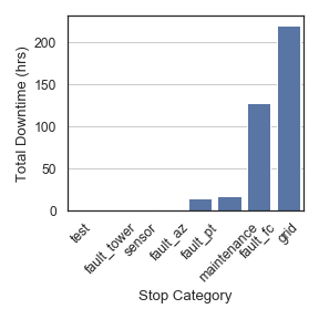
Getting the batch data allows for more complex analysis. Below, the total duration of every stop category in the batches is plotted:
>>> durations = batch_data.groupby(
...     'batch_cat').down_dur.sum().reset_index().sort_values(by='down_dur')
>>> durations.down_dur = durations.down_dur.apply(
...     lambda x: x / np.timedelta64(1, 'h'))
>>> sns.set(font_scale=1.2)
>>> sns.set_style('white')
>>> fig, ax = plt.subplots(figsize=(4, 3))
>>> g = sns.barplot(data=durations, x='batch_cat', y='down_dur', ax=ax,
...                 color=sns.color_palette()[0])
>>> g.set_xticklabels(g.get_xticklabels(), rotation=40)
>>> ax.set(xlabel='Stop Category', ylabel='Total Downtime (hrs)')
>>> ax.yaxis.grid()
Labelling the SCADA data
Once the stoppages have been identified, the data can be labelled for
prognosis or other analysis. This is achieved in the
wtphm.pred_processing module.
The wtpum.pred_processing.label_stoppages() function provides a number of
ways of labelling the scada_data.
For example, suppose we want to label the some specific stoppages in the SCADA
data:
>>> fault_batches = batch_data.loc[[20, 21]]
>>> fault_batches[
...     ['turbine_num', 'fault_root_codes', 'start_time', 'down_end_time',
...      'down_dur', 'repair']]
    turbine_num     fault_root_codes          start_time       down_end_time down_dur  repair
20           22  (68, 113, 144, 500) 2015-12-16 10:00:05 2015-12-16 11:09:07 01:09:02   False
21           22           (144, 500) 2015-12-16 15:03:28 2015-12-16 15:25:42 00:22:14   False
>>>
>>> scada_l = wtphm.pred_processing.label_stoppages(
...     scada_data, fault_batches, drop_fault_batches=False,
...     label_pre_stop=False)
>>> start = fault_batches.start_time.min() - pd.Timedelta('30T')
>>> end = fault_batches.down_end_time.max() + pd.Timedelta('30T')
>>> s_cols = ['time', 'turbine_num', 'stoppage', 'pre_stop', 'batch_id']
>>> scada_l.loc[(scada_l.time >= start) & (scada_l.time <= end) &
...             (scada_l.turbine_num == 22), s_cols]
                    time  turbine_num  stoppage  batch_id
6424 2015-12-16 09:40:00           22         0        -1
6425 2015-12-16 09:50:00           22         0        -1
6426 2015-12-16 10:00:00           22         0        -1
6427 2015-12-16 10:10:00           22         1        20
6428 2015-12-16 10:20:00           22         1        20
6429 2015-12-16 10:30:00           22         1        20
6430 2015-12-16 10:40:00           22         1        20
6431 2015-12-16 10:50:00           22         1        20
6432 2015-12-16 11:00:00           22         1        20
6433 2015-12-16 11:10:00           22         1        20
6434 2015-12-16 11:20:00           22         0        -1
6435 2015-12-16 11:30:00           22         0        -1
6436 2015-12-16 11:40:00           22         0        -1
6437 2015-12-16 11:50:00           22         0        -1
...                  ...          ...       ...       ...
6455 2015-12-16 14:50:00           22         0        -1
6456 2015-12-16 15:00:00           22         0        -1
6457 2015-12-16 15:10:00           22         1        21
6458 2015-12-16 15:20:00           22         1        21
6459 2015-12-16 15:30:00           22         1        21
6460 2015-12-16 15:40:00           22         0        -1
6461 2015-12-16 15:50:00           22         0        -1
In addition, the times leading up to the stoppages can be labelled in the scada data, and the times during the stoppages themselves removed. This is useful for identifying “pre-stop” periods. Here, the times between 30 minutes before and 10 minutes before a fault are labelled as “pre-stop” periods.
>>> scada_l = wtphm.pred_processing.label_stoppages(
...     scada_data, fault_batches, drop_fault_batches=True,
...     label_pre_stop=True, pre_stop_lims=['30 minutes', '10 minutes'])
>>> start = fault_batches.start_time.min() - pd.Timedelta('60T')
>>> s_cols = ['time', 'turbine_num', 'stoppage', 'pre_stop', 'batch_id']
>>> scada_l.loc[(scada_l.time >= start) & (scada_l.time <= end) &
...             (scada_l.turbine_num == 22), s_cols]
                    time  turbine_num  stoppage  pre_stop  batch_id
6421 2015-12-16 09:10:00           22         0         0        -1
6422 2015-12-16 09:20:00           22         0         0        -1
6423 2015-12-16 09:30:00           22         0         0        -1
6424 2015-12-16 09:40:00           22         0         1        20
6425 2015-12-16 09:50:00           22         0         1        20
6426 2015-12-16 10:00:00           22         0         0        20
6434 2015-12-16 11:20:00           22         0         0        -1
...                  ...          ...       ...       ...       ...
6452 2015-12-16 14:20:00           22         0         0        -1
6453 2015-12-16 14:30:00           22         0         0        -1
6454 2015-12-16 14:40:00           22         0         1        21
6455 2015-12-16 14:50:00           22         0         1        21
6456 2015-12-16 15:00:00           22         0         0        21
6460 2015-12-16 15:40:00           22         0         0        -1
6461 2015-12-16 15:50:00           22         0         0        -1
Note that the times of the actual faults have been dropped from the data. This function can also drop additional batches from the SCADA data, so that, e.g. only times leading up to a specific type of fault are included, whereas all other stoppages are removed from the data. This is useful for building or simulating normal behaviour models.
The wtphm.pred_processing also has a function
wtphm.pred_processing.get_lagged_features().
This is useful for classification, and allows features from time \(t - T\)
to be incorporated at time \(t\).
References
| [1] | (1, 2, 3) Leahy, K., Gallagher, C., O’Donovan, P., Bruton, K. & O’Sullivan, D. T. (2018), ‘A Robust Prescriptive Framework and Performance Metric for Diagnosing and Predicting Wind Turbine Faults based on SCADA and Alarms Data with Case Study’, Energies 11(7), pp. 1–21. |
| [2] | Leahy, K., Gallagher, C., O’Donovan, P., & O’Sullivan, D. T. J. (2019), ‘Issues with Data Quality for Wind Turbine Condition Monitoring and Reliability Analyses’, Energies, 12(2):201; https://doi.org/10.3390/en12020201 |
| [3] | Leahy, K., Gallagher, C., O’Donovan, P. & O’Sullivan, D. T. (2018), ‘Cluster analysis of wind turbine alarms for characterising and classifying stoppages’, IET Renewable Power Generation 12(10), 1146–1154. |
| [4] | Qiu, Y., Feng, Y., Tavner, P., Richardson, P., Erdos, G. & Chen, B. (2012), ‘Wind turbine SCADA alarm analysis for improving reliability’, Wind Energy 15(8), 951–966. |